Residual Streams

Introduction

Residual streams (Srivastava et al., 2015) are a key component of the transformer architecture (Vaswani et al., 2017) and are common in deep convolutional neural networks (He et al., 2015). The skip connections between layers allow gradients to propagate backwards through the model efficiently. Karpathy describes residual streams as a way to optimise all the lines of a short program in parallel (Fridman et al., 2022), which I like a lot.

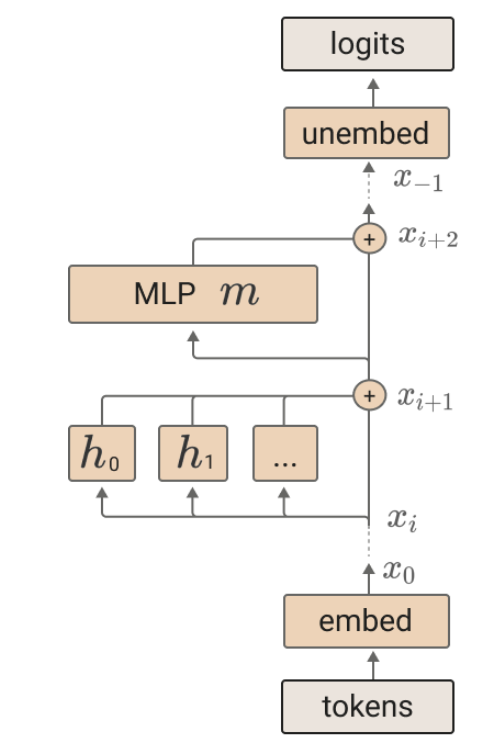
Operations on residual streams are often characterised as reads and writes. This communication is a key component of the stream, which acts as a shared, bottlenecked memory between layers and allows modules to iteratively refine a set of shared features into more specialised ones for prediction. One downside of this approach is that small changes to parameters early in the model could be amplified in later layers and a module that reads from the stream later may expect a different distribution after the update. This problem is overcome with normalisation: batch normalisation in CNNs and layer normalisation in transformers.

Definitions

Before continuing, I must address the confusing terminology as “layer” has specific meanings for each model. Each of the transformers is made up of 12 or 24 layers, each of which is a single residual block. A ResNet is made up of 5 layers containing between 2 and 36 blocks each. On the charts, I plot progression in blocks and have vertical lines showing the separation of layers between ResNet layers.

Another piece of confusing terminology is “features”. Features are properties of the data (dog ears, circles, curves, the texture of broccoli, etc) and some features may not appear in a certain dataset (there are no dog ears in MNIST). Activations are properties of the model when certain data is passed through it - they occur after an operation (add, ReLU, attention, etc) and can be viewed at different resolutions (per neuron, channel, etc).

ResNet Feature Visualisation

Starting with an up-close inspection of image networks, I want to highlight some neuron activations seen under the OpenAI Microscope (Schubert et al., 2020). The initial visualisation is channel 1594 of layer 4 block 3 from ResNet-50 (Figure 2). The choice is fairly arbitrary but is part of some exploration I was doing on the model. From the weights of the last layer, we can see that this channel has the highest contribution to the final probability for class 1 (goldfish). Backtracking through the blocks In the final layer, this feature has been refined into a more and more goldfish-like feature until it makes the final classification (see this notebook for more details).

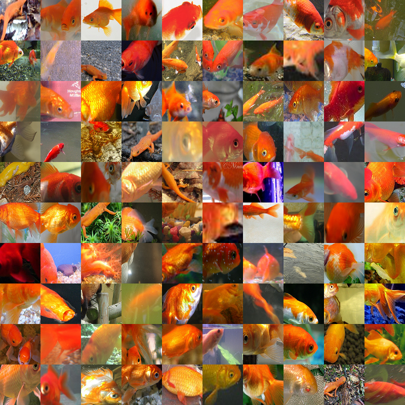
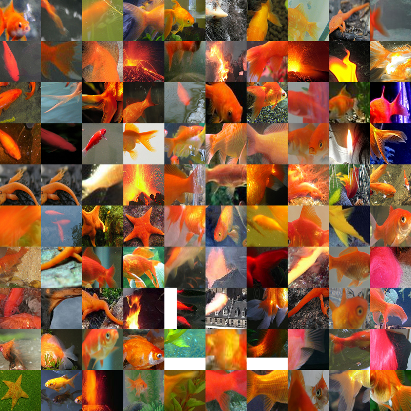
This is my first attempt at an interactive visualisation (Figure 2) in a blog post so it's fairly primitive but I encourage you to visualise different channels so that you have more intuition about the results later. All of the remaining charts give layer-by-layer overviews, however, the visualisations are a useful part of interpreting and understanding neural networks, especially when combined with other approaches (Olah et al., 2017).

It is worth noting that the dimensionality of the residual stream changes between layers in the ResNet due to the down-sampling (Figure 3). The number of channels (which are averaged to identify activations) increases at these points even though the size of the image decreases. This gives some interesting phenomena that transformers (where the residual stream is a fixed size) do not exhibit. The first phenomenon is that there are sharp changes in how features are represented. The type change (Olah, 2015) on these boundaries is dominated by the write from the block rather than the direct shortcut in the residual stream meaning the features do not line up as expected.

Head-Tail Ablation

A further example of the importance of the blocks around layer transitions comes from an experiment where we consider the accuracy of models as we ablate more and more blocks from the start or end (Figure 4). There are very sharp changes in the accuracy of image models when we exclude downsampling blocks, suggesting that these blocks are more important than the blocks around them when modifying the residual stream. Interestingly, we also see a similar phenomenon with layer 20 of RoBERTa-large (Liu et al., 2019) and layer 9 of RoBERTa-base even though the layers are identical (apart from the parameters). This remains a mystery to me and could possibly be an artefact of fine-tuning the model.

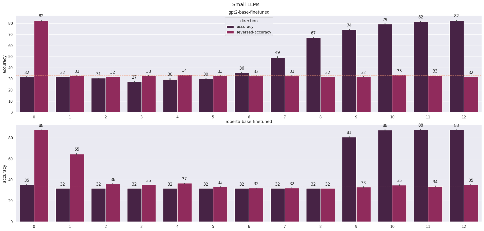
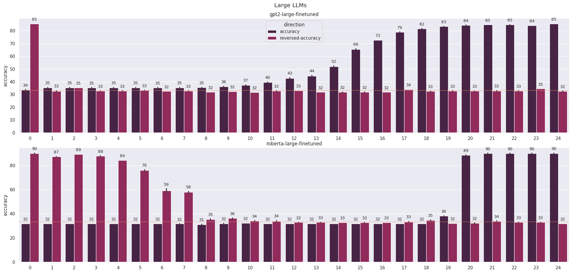
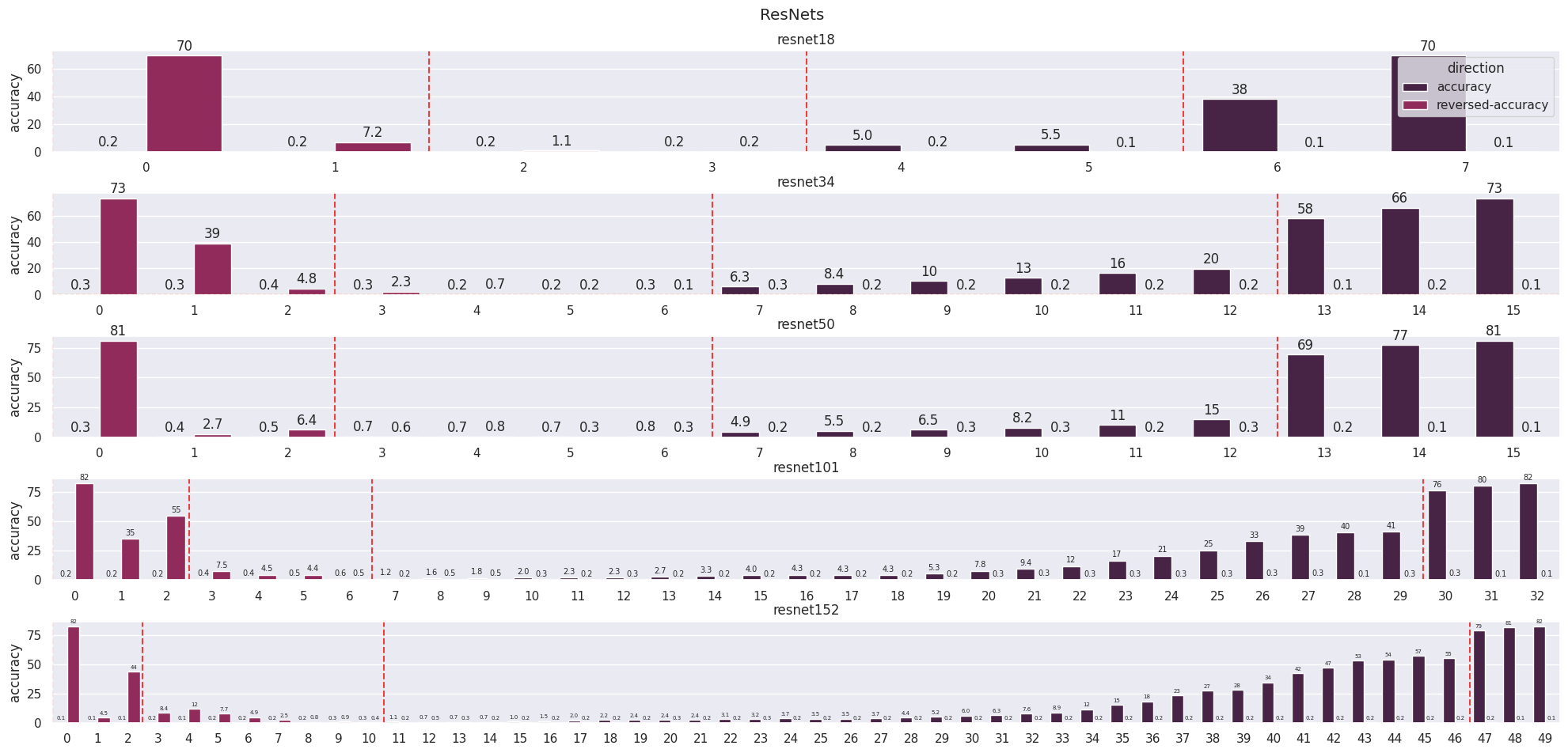
The other clear result from this experiment - that ablating from the end has a less significant effect than ablating from the start - is hardly surprising. Intuitively, we expect that a layer with a different input distribution than expected will magnify this change with an even more anomalous output distribution. These results can also be explained in terms of reads and writes by considering a later layer attempting to read a value that was not written to by a previous one.

Perhaps the most surprising result, however, is that we can ablate so many layers from the end without significant drops in performance, a core concept behind the logit lens (Nostalgebraist, 2021). This really demonstrates the power of the stream as the modules focus on refining the features rather than copying them. One result that I have not shown is that removing the residual stream at any point destroys the network’s performance - it really serves as the spine for these models.

Privileged Basis

We can think of features as being represented by directions (Elhage et al., 2022) and when these directions align with the basis, they become easier to interpret. This phenomenon is known as an aligned basis and may occur when the basis is privileged: components of the setup encourage features to align with the basis and neuron activations to coincide with features. The likelihood of an aligned basis without a privileged basis is negligible so we can use an aligned basis as strong evidence for a privileged basis.

For transformers, the residual stream is generally considered not to be privileged because we only ever perform addition (not an activation) to it, however, for image models, all blocks perform ReLU immediately before adding which creates the privileged basis. Looking at activations, we see neurons and channels give rise to features that align with the basis. To investigate this further, I reproduced some experiments from (Elhage et al., 2023), hoping the presence of an aligned basis may offer some explanations about how the residual stream is used and come to a conclusion about what else is contributing to the privileged basis.

Outliers

Like the original paper, we measure the number of activations where outliers occur in a neuron or channel on the validation set in each layer. The number of outliers is low at the start and increases as we go from generic to specific features, with a change in distribution as we approach the final linear layer. Even with different thresholds, the number of outliers in GPT-2 (Radford et al., 2019) is much larger than in RoBERTa (Liu et al., 2019). This is a byproduct of architecture choices as RoBERTa has a single layernorm at the end of each block, whereas GPT-2 has two in different locations. As in (Dettmers et al., 2022), we see a dichotomy between lots of outliers and very few outliers in the language models (this phenomenon was even more extreme when the standard value of 6 was used as a threshold for outliers).

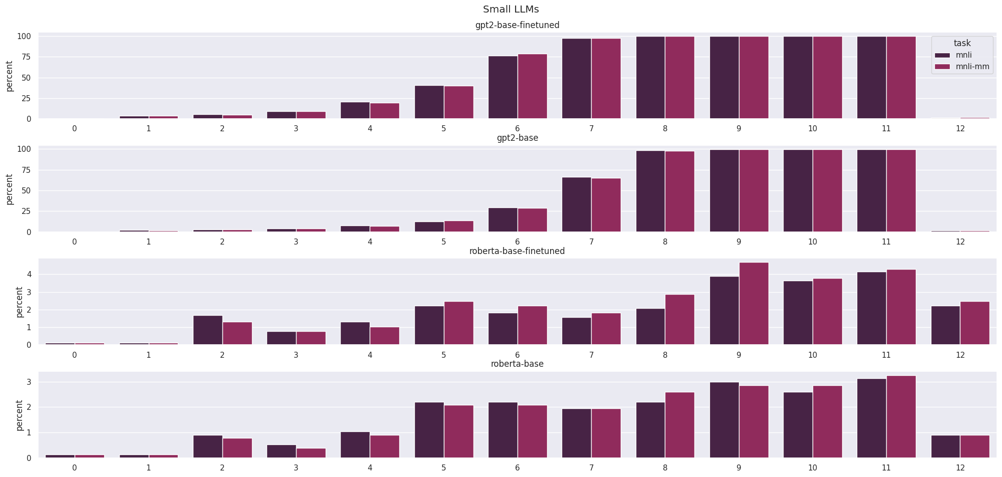
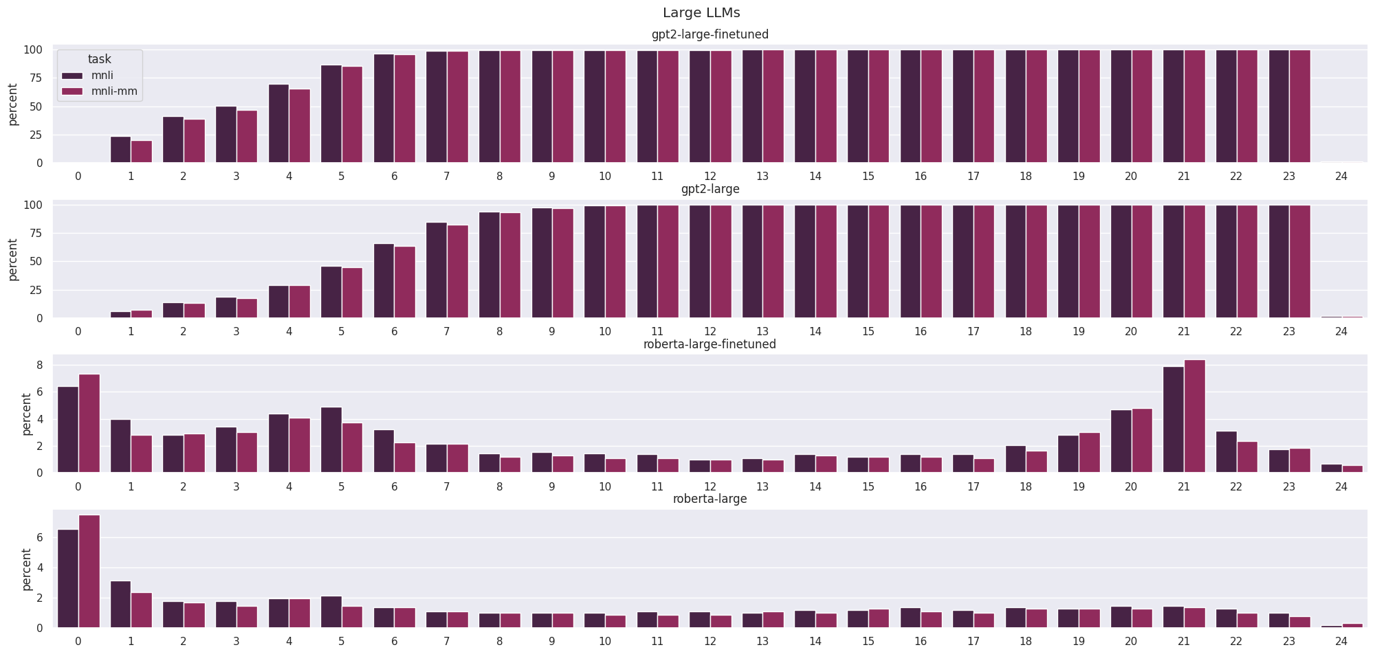
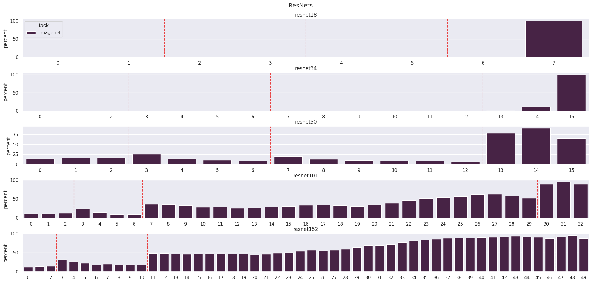
In image models, we see far fewer outliers at the start of the model where features are generic (curve detectors, high-low frequency detectors, etc) and then this increases drastically as we obtain more specific, class-dependent features (dog ears, goldfish, etc). And the change between different numbers of channels is even more drastic given the ability to represent a larger number of complex features.

Kurtosis

Before showing the results of the kurtosis experiments, I will give a short explanation of what it is in case you’re not familiar. Firstly, here is the definition: $$\text{Kurt}\left[X\right] = E\left[\left(\frac{x-\mu}{\sigma}\right)^4\right]$$ The fourth power means that values within 1 standard deviation of the mean have a minimal contribution relative to the values outside. Intuitively kurtosis can be thought of as a measure of the tendency to produce outliers (Westfall, 2014).

If the features are randomly sampled from an isotropic Gaussian distribution, we would expect a kurtosis of 3 in a non-privileged basis (Gaussian distributions have a kurtosis of 3). Isotropic Gaussians are invariant to orthonormal changes of basis so if we take a privileged basis and apply a fixed random rotation to all the features, we can expect the components to be Gaussianly distributed. We verify this to obtain high kurtoses in the aligned basis (no rotation) and kurtoses of approximately 3 in the random basis (rotated) (Figure 6).

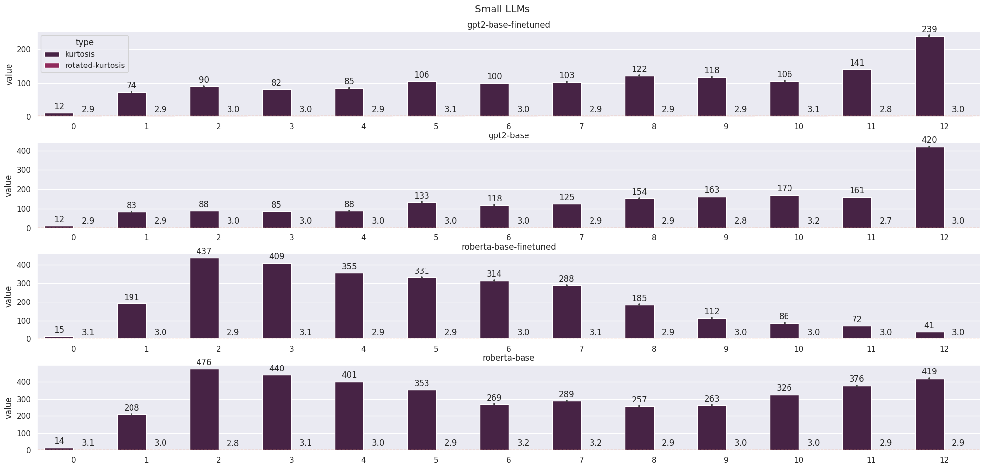
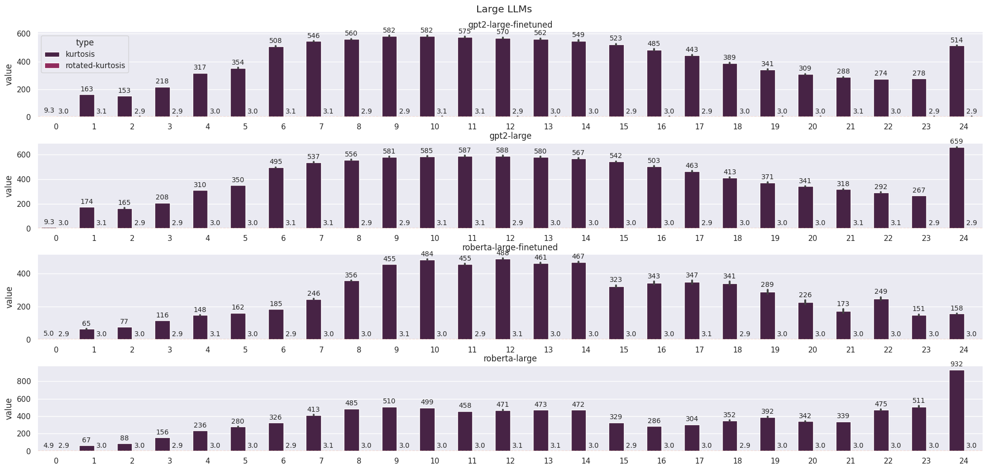
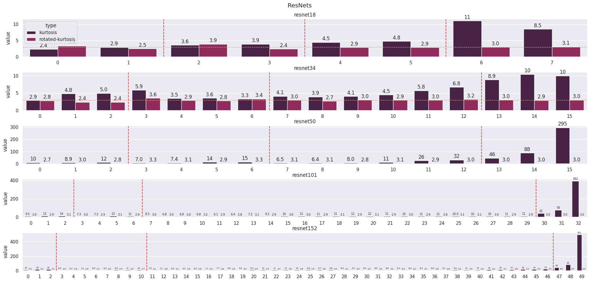
In language models, we already see an aligned basis appearing in the embeddings (layer 0) and we see an interesting range of distributions across the models. Something similar happens in large vision models, however, the values of the kurtoses are smaller.

Effect of the Optimizer

The residual stream is evidently an important part of these model architectures, however, we want to understand why it appears. (Elhage et al., 2023) suggests that this could be due to the layernorm and replaces it with RMSNorm, which is basis invariant. $$\text{RMSNorm}(x_i) = \alpha \cdot \frac{x_i}{\sqrt{\frac 1d \sum_{i=1}^d x_i^2}}$$ They also consider the effects of performing the computation in a separate basis to the stream and this is effective when the computation is different for each head but fails to reduce the kurtosis when the computation basis is shared. In fact, removing all parts of the architecture that could contribute to the alignment doesn’t reduce the kurtosis.

One remaining theory for the presence of the privileged basis is the effect of the optimizer. Firstly, I train a ResNet with SGD to gain some intuitions about whether doing so with a transformer will be worthwhile. I obtain reasonable accuracy after training ResNet-18 and ResNet-34 (with RMSNorm over BatchNorm) on ImageNet (Russakovsky et al., 2015) for 20 epochs but these models are much more fragile (Figure 7). The kurtosis remains high, as expected (Figure 8).

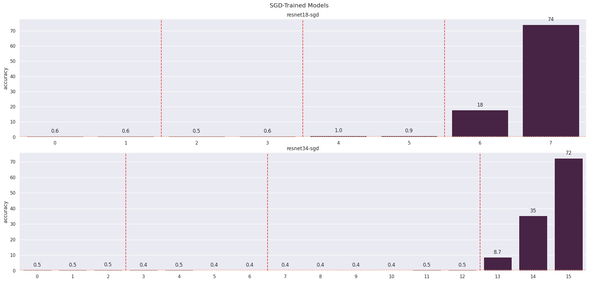
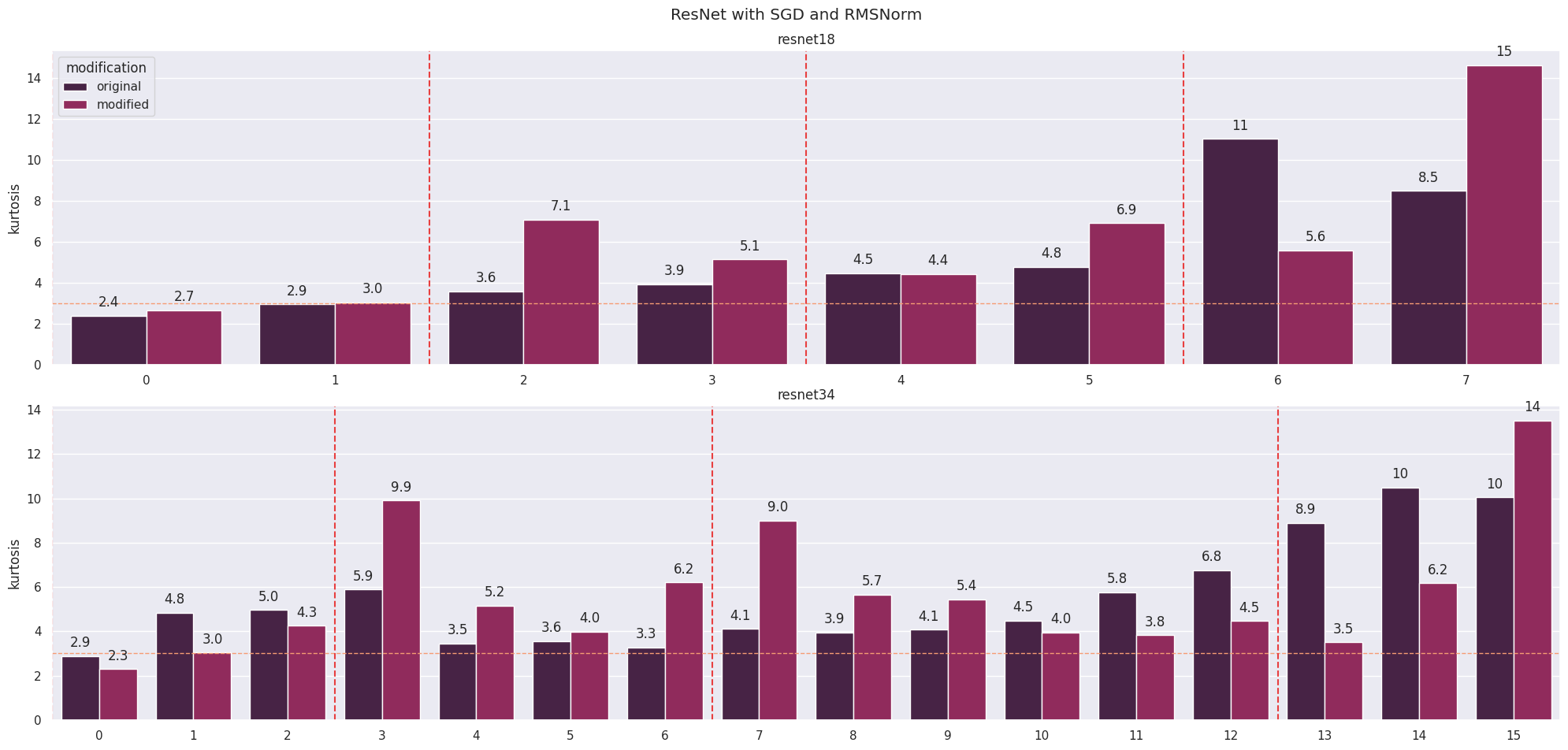
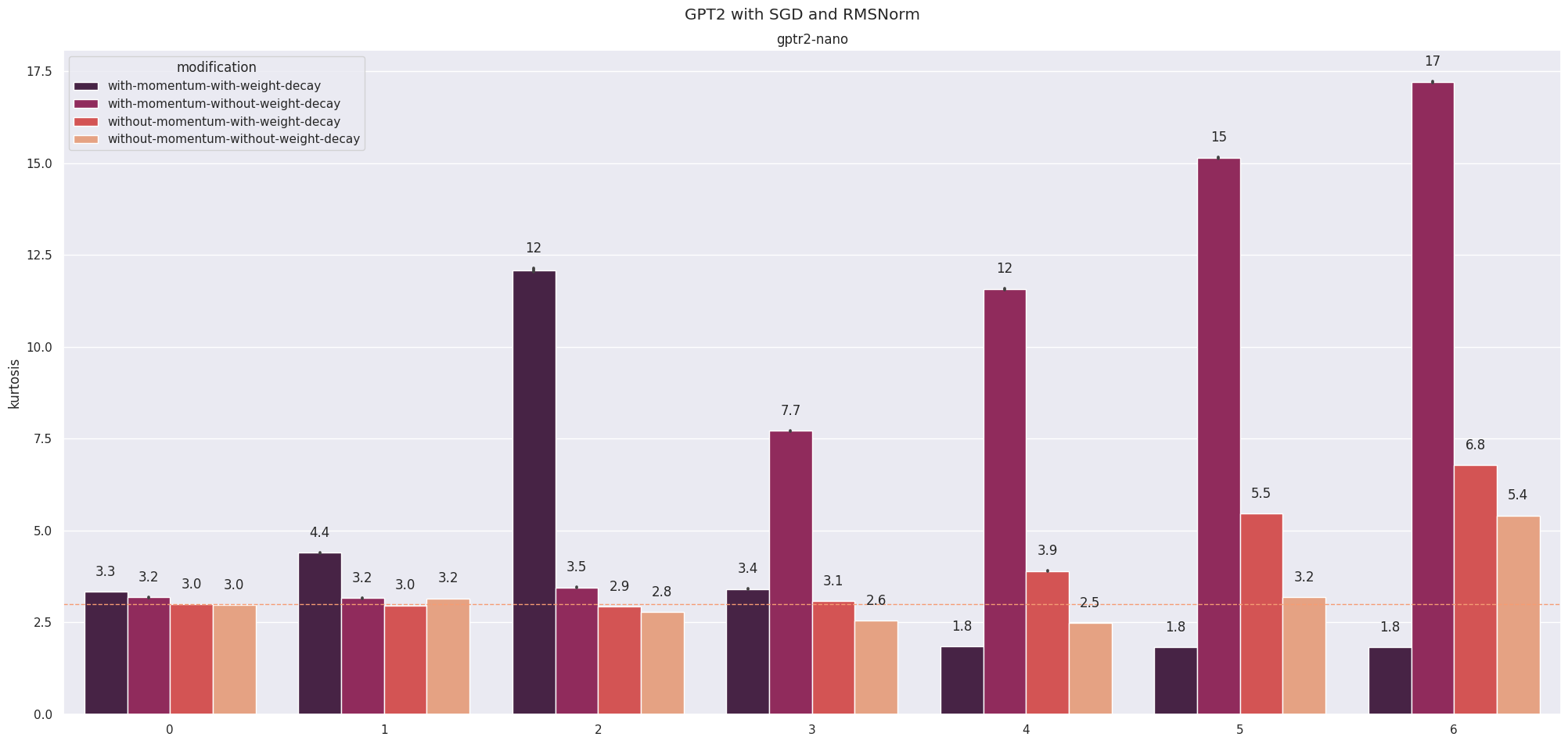
I run a similar setup with “gptr2-nano” (Sharkey et al., 2022), a GPT-2 style architecture with 6 layers and 4 heads but with RMSNorm instead of LayerNorm trained for one epoch on Wikipedia. I train models using gradient clipping (the RMSNorm weight was diverging) with and without momentum and weight decay (four models in total) and measure the resulting kurtoses.

The results are surprising but inconclusive. The model that is closest to having a kurtosis of 3 in all layers is the model trained without weight decay or momentum. However, we see a divergence from this in the final layer, which doesn’t quite match the results from a model trained with independent rotations (Elhage et al., 2023). The kurtosis is also 3 for the first three layers of the model trained without momentum but with weight decay, which is also promising, but this changes towards the end of the model. The strangest result (to me at least) is that the model trained with momentum and without weight decay has an increasing kurtosis but drops to less than 3 in the final three layers, suggesting a very different distribution from what we’d expect. Although not shown, the kurtosis is approximately three for all of these models in a randomly rotated basis.

Conclusions

Residual streams are an extremely important part of the transformer and ResNet architectures with modules reading to and writing to it as a shared memory. Under conventional training schemes, they form a privileged basis, which produces aligned, interpretable features that give more of an insight into how the network operates.

We assume the distribution of the activations of the residual stream is Gaussian in a random basis and see strong evidence for this. In teh original basis, however, it has a much higher kurtosis than we would expect - strong evidence for an aligned basis. We can recover the Gaussianness by rotating into a random basis but changes to the architecture alone do not restore a kurtosis of 3. However, we have found evidence that the optimizer is responsible for the aligned basis. With an undertrained, small model, it is impossible to say this for certain but I pass on the baton for someone to repeat these experiments, as I expect that this can be solved with more data and more compute (Sutton, 2019).

Code

The code is available on GitHub: https://github.com/George-Ogden/residual-streams

Bibliography

R.Srivastava, K.Greff, JürgenSchmidhuber. Highway Networks. arXiv preprint arXiv:1505.00387, 2015.
A.Vaswani, N.Shazeer, N.Parmar, J.Uszkoreit, L.Jones, A.Gomez, L.Kaiser, I.Polosukhin. Attention Is All You Need. arXiv preprint arXiv:1706.03762, 2017.
K.He, X.Zhang, S.Ren, J.Sun. Deep Residual Learning for Image Recognition. arXiv preprint arXiv:1512.03385, 2015.
L.Fridman, A.Karpathy. #333 – Andrej Karpathy: Tesla AI, Self-Driving, Optimus, Aliens, and AGI. Lex Fridman Podcast, 2022.
L.Schubert, M.Petrov, S.Carter. OpenAI Microscope. OpenAI Blog, 2020.
C.Olah, A.Mordvintsev, L.Schubert. Feature Visualization. Distill, 2017.
C.Olah. Neural networks, types, and functional programming. Neural Networks, Types, and Functional Programming -- colah's blog, 2015.
Y.Liu, M.Ott, N.Goyal, J.Du, M.Joshi, D.Chen, O.Levy, M.Lewis, L.Zettlemoyer, V.Stoyanov. RoBERTa: {A} Robustly Optimized {BERT} Pretraining Approach. arXiv preprint arXiv:1907.11692, 2019.
Nostalgebraist. Interpreting GPT: The logit lens. LessWrong, 2021.
N.Elhage, T.Hume, C.Olsson, N.Schiefer, T.Henighan, S.Kravec, Z.Hatfield-Dodds, R.Lasenby, D.Drain, C.Chen et al.. Toy Models of Superposition. Anthropic, 2022.
N.Elhage, R.Lasenby, C.Olah. Privileged Bases in the Transformer Residual Stream. Anthropic, 2023.
A.Radford, J.Wu, R.Child, D.Luan, D.Amodei, I.Sutskever. Language Models are Unsupervised Multitask Learners. Preprint 2019, 2019.
T.Dettmers, M.Lewis, Y.Belkada, L.Zettlemoyer. LLM.int8(): 8-bit Matrix Multiplication for Transformers at Scale. CoRR, 2022.
P.Westfall. Kurtosis as Peakedness, 1905–2014. R.I.P.. The American Statistician, 2014.
O.Russakovsky, J.Deng, H.Su, J.Krause, S.Satheesh, S.Ma, Z.Huang, A.Karpathy, A.Khosla, M.Bernstein et al.. {ImageNet Large Scale Visual Recognition Challenge}. International Journal of Computer Vision (IJCV), 2015.
L.Sharkey, D.Braun, B.Millidge. [Interim research report] Taking features out of superposition with sparse autoencoders. AI Alignment Forum, 2022.
R.Sutton. The Bitter Lesson. The Bitter Lesson, 2019.
N.Elhage, N.Nanda, C.Olsson, T.Henighan, N.Joseph, B.Mann, A.Askell, Y.Bai, A.Chen, T.Conerly et al.. A Mathematical Framework for Transformer Circuits. Anthropic, 2023.
N.Cammarata, S.Carter, G.Goh, C.Olah, M.Petrov, L.Schubert. Thread: Circuits. Distill, 2020.